PyTorch’s Dynamic Graphs (Autograd)
The acyclical graphs design powering modern deep learning frameworks
One brilliant engineering innovation implemented by PyTorch (of which there are many) is its dynamic graphs.
Torch’s magic is its automatic differentiation engine torch.autograd— able to compute gradients and optimize parameters efficiently.
Under the hood, autograd contains some awesome engineering, all tied together by its graphical data structure.
Neural Network
Consider a simple torch neural net to demonstrate. The model code is taken from PyTorch documentation.
Data
Load the modules and data. Torch uses a Dataloader module to wrap an instance of its datasets class for sampling/shuffling.
from torchvision.transforms import ToTensor
from torch.utils.data import DataLoader
from torchvision import datasets
from torchviz import make_dot
from torch import nn


# Download training data from open datasets.
training_data = datasets.FashionMNIST(root="data",
    train=True,
    download=True,
    transform=ToTensor(),
)

# Download test data from open datasets.
test_data = datasets.FashionMNIST(
    root="data",
    train=False,
    download=True,
    transform=ToTensor(),
)

batch_size = 64

# Create data loaders.
train_dataloader = DataLoader(training_data, batch_size=batch_size)
test_dataloader  = DataLoader(test_data, batch_size=batch_size)

for X, y in test_dataloader:
    print(f"Shape of X [N, C, H, W]: {X.shape}")
    print(f"Shape of y: {y.shape} {y.dtype}")
    break

device = (
    "cuda"      if torch.cuda.is_available()
    else "mps"  if torch.backends.mps.is_available()
    else "cpu"
)
print(f"Using {device} device")
Shape of X [N, C, H, W]: torch.Size([64, 1, 28, 28])
Shape of y: torch.Size([64]) torch.int64
Using mps device
Network
A PyTorch model inherits from nn.Module, and implements a constructor __init__(self) and the forward pass through the model/prediction space forward.
Note: A PyTorch model is usually a Neural Net. However, in actuality, it’s any module that inherits from torch.nn.Module that couples data and transformations, holding the methods to initiate the model structure self.__init__() and transform the data self.forward().
# define model
class NeuralNetwork(nn.Module):
  def __init__(self):
    super().__init__()
    self.flatten = nn.Flatten()
    self.linear_relu_stack = nn.Sequential(
      nn.Linear(28*28, 512),
      nn.ReLU(),
      nn.Linear(512, 512),
      nn.ReLU(),
      nn.Linear(512, 10),
  )

  def forward(self, x):
    x       = self.flatten(x)
    logits  = self.linear_relu_stack(x)
    return logits

model = NeuralNetwork().to(device)
print(model)
NeuralNetwork(
(flatten): Flatten(start_dim=1, end_dim=-1)
(linear_relu_stack): Sequential(
(0): Linear(in_features=784, out_features=512, bias=True)
(1): ReLU()
(2): Linear(in_features=512, out_features=512, bias=True)
(3): ReLU()
(4): Linear(in_features=512, out_features=10, bias=True)
)
)
Generate model schematic:
model.eval()
X     = torch.randn(1, 1, 28, 28).to(device)
pred  = model(X)
make_dot(pred, params=dict(list(model.named_parameters()))).render("rnn_torchviz", format="png")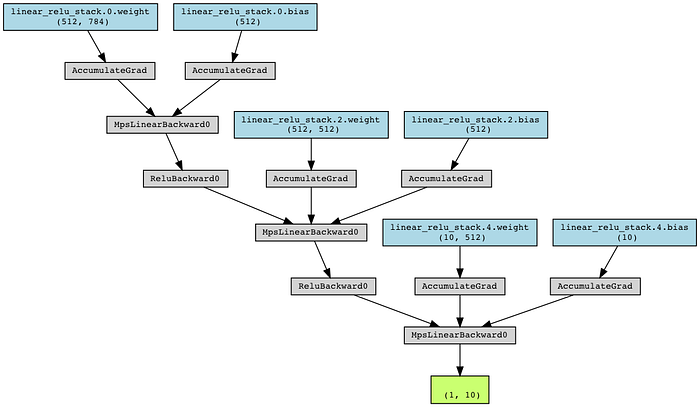
Fitting the model
# Initialize the loss function
loss_fn   = nn.CrossEntropyLoss()
optimizer = torch.optim.SGD(model.parameters(), lr=1e-3)

# Training loop
def train_loop(dataloader, model, loss_fn, optimizer):
    size = len(dataloader.dataset)
    model.train()
    for batch, (X, y) in enumerate(dataloader):
        # Compute prediction and loss
        pred = model(X)
        loss = loss_fn(pred, y)

        # Backpropagation
        loss.backward()
        optimizer.step()
        optimizer.zero_grad()

        if batch % 100 == 0:
            loss, current = loss.item(), batch * len(X)
            print(f"loss: {loss:>7f}  [{current:>5d}/{size:>5d}]")

# Evaluation loop
def test_loop(dataloader, model, loss_fn):
    size = len(dataloader.dataset)
    model.eval()
    num_batches = len(dataloader)
    test_loss, correct = 0, 0

    # ensures no gradients are computed during test mode
    with torch.no_grad():
        for X, y in dataloader:
            pred = model(X)
            test_loss += loss_fn(pred, y).item()
            correct += (pred.argmax(1) == y).type(torch.float).sum().item()

    test_loss /= num_batches
    correct /= size
    print(f"Test Error: \n Accuracy: {(100*correct):>0.1f}%, Avg loss: {test_loss:>8f} \n")


# Fit the model
epochs = 25
for t in range(epochs):
    print(f"Epoch {t+1}\n-------------------------------")
    train_loop(train_dataloader, model, loss_fn, optimizer)
    test_loop(test_dataloader, model, loss_fn)
print("Done!")
This demonstrates the full optimization procedure in practice. We can slice out a single node from our neural net to get a clearer understanding.
Single Node: Lower Level Implementation

Our parameter set & transformations are initialized by the torch.nn API calls (nn.Sequential). Consider a single node in the neural network, this could be implemented:
import torch

x = torch.ones(5)   # input tensor
y = torch.zeros(3)  # expected output
w = torch.randn(5, 3, requires_grad=True)
b = torch.randn(3, requires_grad=True)
z = torch.matmul(x, w)+b
loss = torch.nn.functional.binary_cross_entropy_with_logits(z, y)
Autograd
Now that our node is set up, there are a few things to notice about the training/testing implementation.
Computing Gradients
We compute the derivates of our loss function with respect to all flagged parameters in the backward() pass through our network.
loss.backward()
print(w.grad)
print(b.grad)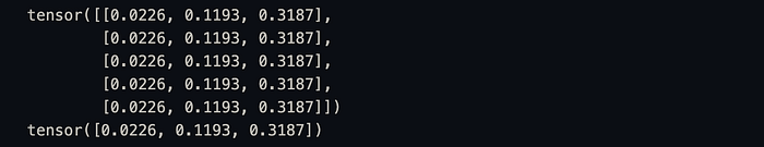
Note: optimizer.zero_grad() is used in our training function to ensure gradients do not accumulate, which would destabilise our optimization procedure.
Gradient Tracking
- In our lower-level implementation, trainable parameters are flagged using the
requires_grad=Trueparameter. This is how Torch keeps track of which gradients to calculate & (back)-propagate. - Gradients of the
lossfunction are calculated wr.t variables flaggedrequires_grad=True.
Note: The requires_grad flag can be changed at any stage on any parameter. This is crucial to Torch‘s usability. This allows us to freeze parameters and implement more efficient forward passes during the inference stage.
z = torch.matmul(x, w)+b
print(z.requires_grad)

with torch.no_grad():
    z = torch.matmul(x, w)+b
print(z.requires_grad)

# alternatively one can use `.detach()`
z = torch.matmul(x, w)+b
z_det = z.detach()
print(z_det.requires_grad)
Computational Graph (DAG)
PyTorch builds a computational graph dynamically at runtime to store the connections between parameters and gradients.
A directed acyclic graph (DAG) is used to keep track of the data (tensors), all data transformations (operations) and the output tensors.
Backpropagation traverses the DAG in reverse to compute gradients, starting from the leaf nodes.
Dynamicity & Control Flow
Each iteration in the training loop constructs a new computational graph as data is fed through the model, the graph is dynamic as it changes based on specific data and operations performed in that iteration. This allows us to inject control flow and build any arbitrary function as a model — providing incredible flexibility.
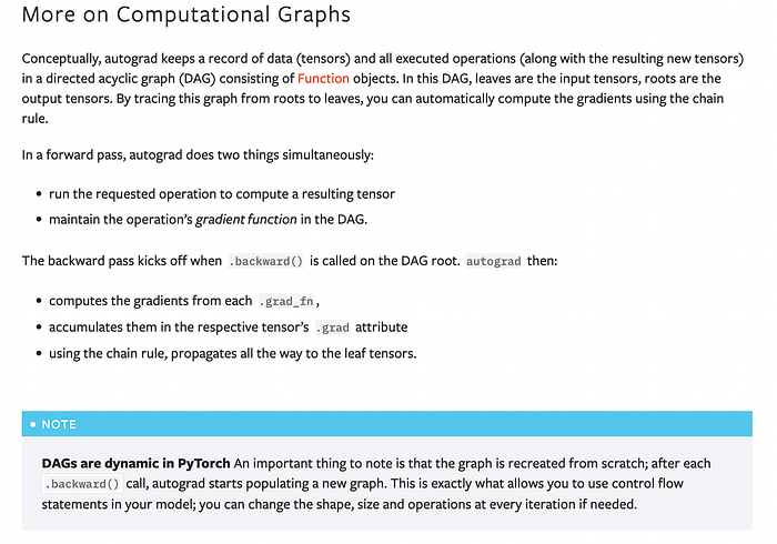
Constructing the DAG
The DAG’s leaves are in the input tensors and the roots are the output tensors. By tracing the graph from roots to leaves, gradients are computed using the chain rule.
The DAG is not built explicitly but is rather represented by a series of nodes and edges implicit in the training process.
Read more on Autograd’s mechanics here.
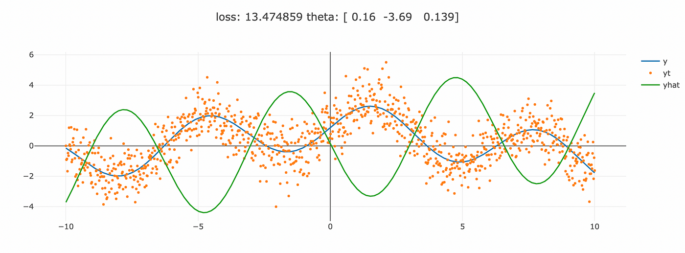
Consider a final example to demonstrate the DAG. Here we sample y as a function of X. The (unknown) data-generating process is given by:

import plotly.graph_objects as go
import plotly.express as px
from torch import nn
import numpy as np
import torch
import math

# data generating process
X  = torch.tensor(np.linspace(-10, 10, 1000))
y  = 1.5 * torch.sin(X) + 1.2 * torch.cos(X/4)
yt = y + np.random.normal(0, 1, 1000)

# vis
def plotter(X, y, yhat=None, title=None):
  with torch.no_grad():
    fig = go.Figure()
    fig.add_trace(go.Scatter(x=X, y=y, mode='lines',    name='y'))
    fig.add_trace(go.Scatter(x=X, y=yt, mode='markers', marker=dict(size=4), name='yt'))
    if yhat: fig.add_trace(go.Scatter(x=X, y=yhat, mode='lines', name='yhat'))
    fig.update_layout(template='none', title=title)
    fig.show()

plotter(X, y, title='Data Generating Process')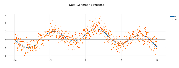
We then write a function to fit a model to the data, given a set of parameters. This could parameterise a neural network, however, we’ll use a simpler sinusoidal model. Further, define the parameter space & optimization procedure here. Finally, we instantiate a training loop.
# build model
def fit_model(theta:torch.tensor=torch.rand(3, requires_grad=True)):
    return theta[0] * X + theta[1] * torch.sin(X) + theta[2] * torch.cos(X/4)

# params
theta = torch.randn(3, requires_grad=True)

# optimization proce
loss_fn  = nn.MSELoss()                         # MSE loss
optimizer = torch.optim.SGD([theta], lr=0.01)   # build optimizer

# run training
epochs = 500
for i in range(epochs):
  yhat = fit_model(theta)
  loss = loss_fn(y, yhat)
  loss.backward()
  optimizer.step()
  optimizer.zero_grad()
  if i % (epochs/10) == 0:
    msg = f"loss: {loss.item():>7f} theta: {theta.detach().numpy()}"
    yhat = fit_model(theta)
    plotter(X, y, yhat.detach(), title=f"loss: {loss.item():>7f} theta: {theta.detach().numpy().round(3)}")
During training, we periodically log the loss, the parameter values, and plot the model estimates. Running the training loop yields:


Dissecting the DAG:
The state is traversed through our DAG by calling 3 methods:
loss.backward(): computes the gradients oftheta.optimizer.step(): updates the values ofthetaby taking stepping through the optimization procedure.optimizer.zero_grad(): zeros out the gradients to avoid run-away gradients.
Implicitly building our DAG, according to the runtime logic of each epoch.
Summary
PyTorch’s dynamic computational graph offers a number of advantages:
- Flexibility: Allows for the creation of complex, dynamic models that contain control flow, domain/business logic & variable length parameters.
- Memory Efficiency: Constructing the graphs iteratively allows PyTorch to free up memory from previously used but now superfluous graph components — only storing what is essential in a given run.
- Debugging& Logging: Access to real-time data is valuable when debugging or monitoring a program's behaviours.
- Gradient toggling: Gradient tracking and computation can be toggled on and off at runtime. The
torch.no_grad()context manager can be used during inference or to freeze a (sub)set of parameters for transfer learning, meta-learning etc. - Dynamic models: The flexibility also allows the same framework to extend to models with variable parameter, input & output spaces.
- Cleaner code: A static graph would require more Boilerplate Code to define the gradient traversal.
- Ease of Experimentation: Prototyping is straightforward.